Introduction
Overview
Teaching: 5 min
Exercises: 0 minQuestions
How do I run BGCflow in my computer?
Objectives
Getting a copy of BGCflow in your own machine
Welcome to the BGCFlow tutorial! BGCFlow is a stack of bioinformatic tools that enables you to analyze biosynthetic gene clusters (BGCs) across large collections of genomes (pangenomes) using the Snakemake workflow manager. In this tutorial, you will learn how to set up and use BGCFlow to streamline your BGC analysis.
Before you start
Before you dive into using BGCFlow, there are a few prerequisites you need to have in place
Access to a Linux Environment
BGCFlow is currently tested on Linux (specifically Ubuntu 22). If you’re a Windows user, don’t worry, you have options too:
- You can set up a Linux virtual machine (VM) using cloud providers like Microsoft Azure, AWS, or Google Cloud.
- Windows users can also utilize Windows Subsystem for Linux (WSL2) to create a Linux-like environment.
Conda or Mamba Package Manager
BGCflow requires a UNIX based environment with Conda installed. If you’re not familiar with Conda, you can find installation instructions here. Additionally, we recommend considering Mamba, an alternative package manager. If you’re not using Mambaforge, you can install Mamba into any other Conda-based Python distribution with the following command:
conda install -n base -c conda-forge mambaWith these essentials in place, you’re ready to proceed with setting up BGCFlow!
Installing BGCFlow environments
Creating a Conda Environment
Let’s start by creating a dedicated Conda environment for BGCFlow:
# create and activate a new conda environment
mamba create -n bgcflow -c conda-forge python=3.11 pip openjdk -y # also install java for metabase
- PS: This environment includes Java / OpenJDK which is required for serving
metabase.
Installing the BGCFlow wrapper
Next, we’ll install the BGCFlow wrapper, a command-line interface that makes working with BGCFlow’s Snakemake workflows easier:
# activate bgcflow environment
conda activate bgcflow

# install `BGCFlow` wrapper
pip install bgcflow_wrapper

# make sure to use bgcflow_wrapper version >= 0.2.7
bgcflow --version # show the wrapper version

# Verify the installation and view available command line arguments
bgcflow --help
The above command will display the help function of the wrapper, providing a comprehensive list of available command line arguments:
$ bgcflow --help
Usage: bgcflow [OPTIONS] COMMAND [ARGS]...

  A snakemake wrapper and utility tools for BGCFlow
  (https://github.com/NBChub/bgcflow)

Options:
  --version   Show the version and exit.
  -h, --help  Show this message and exit.

Commands:
  build       Build Markdown report or use dbt to build DuckDB database.
  clone       Get a clone of BGCFlow to local directory.
  deploy      [EXPERIMENTAL] Deploy BGCFlow locally using snakedeploy.
  get-result  View a tree of a project results or get a copy using Rsync.
  init        Create projects or initiate BGCFlow config from template.
  pipelines   Get description of available pipelines from BGCFlow.
  run         A snakemake CLI wrapper to run BGCFlow.
  serve       Serve static HTML report or other utilities (Metabase,...
  sync        Upload and sync DuckDB database to Metabase.
Additional pre-requisites
While the wrapper installation covers the basics, there are a few additional steps to ensure smooth operation:
- Adjust Conda Channel Priorities: Set the Conda channel priorities to ‘flexible’ for a more adaptable package resolution:
With the environment activated, install or setup this configurations:
- Set
condachannel priorities toflexibleconda config --set channel_priority disabled conda config --describe channel_priorityWith these steps completed, you’ve laid a solid foundation for using BGCFlow effectively.
- Set
Deploying a local copy of BGCFlow
Before you can start genome mining on your dataset, you’ll need to deploy the BGCFlow workflow locally. Follow the steps below to get BGCFlow set up on your machine.
Cloning BGCFlow Repository
-
Navigate to the directory where you want to store your BGCFlow installation. Make sure you have a decent amount of storage space available.
-
Run the following command to clone the BGCFlow repository to your chosen destination:
bgcflow clone <my BGCFlow folder>Replace
<my BGCFlow folder>with the path to your desired destination directory.
Additionally, you can specify a specific branch or release tags of BGCFlow to clone using the --branch option. By default, the main branch will be cloned.
bgcflow clone --branch v0.8.1 <my BGCFlow folder>
You can also manually grab other releases from the the github repository tags and click on the release/tags of your choice. On the assets, you can click the source code link to download it.
Initiating configuration from template
To run BGCFlow, users need to set up a Snakemake configuration file and the PEP file for each projects. To initiate an example config.yaml from template and run an example project, do:
bgcflow init
You can modify the configuration located in config/config.yaml to point out to the right project PEPs.
projects:
  - name: config/Lactobacillus_delbruecki/project_config.yaml
Running the Lactobacillus tutorial dataset
For the tutorial, we will be running a small dataset of Lactobacillus delbrueckii genomes from NCBI.
You can do a dry-run (checking the workflow without actually running it) using:
bgcflow run -n
When you are ready to run the workflow, remove the -n flag. You can see the full parameters by running bgcflow run --help. For now, let it be and skip to the next section of the tutorial.
Download the latest release/tags
The command bgcflow clone utilizes git to get the latest branch of BGCFlow. You can also grab other releases from the the github repository tags at https://github.com/NBChub/bgcflow/tags and click on the latest release/tags. On the assets, you can click the source code link to download it.
Key Points
A Snakemake environment is required to run BGCflow
bgcflow_wrapperprovides shortcut to commonly used Snakemake commands and other tools integrated in BGCFlow
BGCflow project structure
Overview
Teaching: 5 min
Exercises: 0 minQuestions
How do I set my BGCflow project?
Objectives
Setting up configuration and files to start a BGCflow project
Setting up your Project Config
Let’s move into our freshly cloned BGCflow folder
cd bgcflow
To run BGCFlow, we need to activate the BGCFlow conda environment and invoke the command line interface:
conda activate bgcflow
bgcflow --help
Setting up your project samples
In this tutorial, we will analyse 18 publicly available Streptomyces venezuelae genomes. To do that, we will need to prepare a sample.csv file with a list of the genome accession ids.
Please find the sample.csv for the tutorial here: https://github.com/NBChub/bgcflow_tutorial/blob/gh-pages/files/samples.csv.
This is how the top of the table looks like:
| genome_id | source | organism | genus | species | strain | closest_placement_reference |
|---|---|---|---|---|---|---|
| GCF_000253235.1 | ncbi | ATCC 10712 | ||||
| GCF_001592685.1 | ncbi | WAC04657 | ||||
| … | … | … | … | .. | … | … |
There are two required columns that needs to be filled:
genome_id[required]: The genome accession ids (with genome version forncbiandpatricgenomes). Forcustomfasta file provided by users, it should refer to the fasta file names stored indata/raw/fasta/directory with.fnaextension.source[required]: Source of the genome to be analyzed choose one of the following:custom,ncbi,patric. Where:custom: for user provided genomes (.fna) in thedata/raw/fastadirectory with genome ids as filenamesncbi: for list of public genome accession IDs that will be downloaded from the NCBI refseq (GCF…) or genbank (GCA…) databasepatric: for list of public genome accession IDs that will be downloaded from the PATRIC database
The other optional metadata that we can provide are:
organism[optional] : name of the organism that is same as in the fasta headergenus[optional] : genus of the organism. Ideally identified with GTDBtk.species[optional] : species epithet (the second word in a species name) of the organism. Ideally identified with GTDBtk.strain[optional] : strain id of the organismclosest_placement_reference[optional]: if known, the closest NCBI genome to the organism. Ideally identified with GTDBtk.
For now, we will only provide the strain information and leave the taxonomic information blank. For publicly available genomes, BGCflow will try to fetch the taxonomic placement from GTDB release 202.
To set up the config, we will create a project folder named s_venezuelae inside the config directory:
mkdir -p config/s_venezuelae
wget -O config/s_venezuelae/samples.csv https://raw.githubusercontent.com/NBChub/bgcflow_tutorial/gh-pages/files/samples.csv
Define your project in the config.yaml
Now that we have our sample file ready, we need to define our project in the config.yaml. An example of the config file can be found in the config/examples/_config_example.yaml.
Let’s copy that file and use it as a template:
cp config/examples/_config_example.yaml config/config.yaml
Let’s open the newly created config.yaml. The newly copied config.yaml will have this example project defined:
# Project 1
  - name: example
    samples: config/examples/_genome_project_example/samples.csv
    rules: config/examples/_genome_project_example/project_config.yaml
    prokka-db: config/examples/_genome_project_example/prokka-db.csv
    gtdb-tax: config/examples/_genome_project_example/gtdbtk.bac120.summary.tsv
Replace those lines with this:
# Project 1
  - name: s_venezuelae
    samples: config/s_venezuelae/samples.csv
#    rules: config/examples/_genome_project_example/project_config.yaml
#    prokka-db: config/examples/_genome_project_example/prokka-db.csv
#    gtdb-tax: config/examples/_genome_project_example/gtdbtk.bac120.summary.tsv
For now, we will just use two mandatory variables:
name: name of your projectsamples: a csv file containing a list of genome ids for analysis with multiple sources mentioned. Genome ids must be unique.
PS: Commented lines will not be processed.
Checking the jobs with Snakemake dry-run
Before, we use the -n when calling snakemake. This parameters means a dry-run, which is used to simulate all the jobs that will be run given the information provided in the config file. You can also add the parameters -r to see the reason why those jobs are generated.
Let’s do a dry run to check if our project is successfully configured:
snakemake -n -r
Challenges
- How many jobs will be generated?
- How many
antismashjobs will be generated?- Why do each jobs only run with 1 core?
- What do you think
localrulealldoes?
Key Points
A project requires a PEP configuration and a
.csvfile containing a list of genomes to analyseThe project is then defined in the
config.yamlfileAn example of a project config can be found in
config/examples
Selecting rules for analysis
Overview
Teaching: 5 min
Exercises: 0 minQuestions
How do I set which rules to run?
Objectives
Getting able to select specific BGCflow rules to run
Global Rules
In the previous tutorial, when doing a dry-run, Snakemake will generate this jobs:
Job stats:
job                          count    min threads    max threads
-------------------------  -------  -------------  -------------
all                              1              1              1
antismash                       18              1              1
antismash_db_setup               1              1              1
antismash_summary                1              1              1
downstream_bgc_prep              1              1              1
extract_meta_prokka             18              1              1
extract_ncbi_information         1              1              1
fix_gtdb_taxonomy                1              1              1
format_gbk                      18              1              1
gtdb_prep                       18              1              1
ncbi_genome_download            18              1              1
prokka                          18              1              1
write_dependency_versions        1              1              1
total                          115              1              1
In BGCflow, rules are defined globally in the config.yaml. Rules can be turned on or off by setting the value for each specific rules with TRUE or FALSE.
#### GLOBAL RULE CONFIGURATION ####
# This section configures the rules to run globally.
# Use project specific rule configurations if you want to run different rules for each projects.
# rules: set value to TRUE if you want to run the analysis or FALSE if you don't
rules:
  seqfu: FALSE
  mlst: FALSE
  refseq-masher: FALSE
  mash: FALSE
  fastani: FALSE
  checkm: FALSE
  prokka-gbk: FALSE
  antismash-summary: TRUE
...
Notice that the only rules set to TRUE are antismash-summary. So why does Snakemake generate a total of 115 jobs? That is because to generate the final output of antismash-summary, other job outputs are required. Snakemake will trace back all the file dependency of the final output and call every jobs require to generate that file.
The rule setting in the config.yaml applies globally. So if you several projects that require the same analysis, the rule setting will be applied to all those projects.
Project specific rule
What if I want to run different analysis for each projects? For this application, you can override the global rule setting by giving each project a .yaml file containing project specific rule setting. The file contents is exactly the same as the global rule configuration:
#### RULE CONFIGURATION ####
# rules: set value to TRUE if you want to run the analysis or FALSE if you don't
rules:
  seqfu: TRUE
  mlst: FALSE
  refseq-masher: FALSE
  mash: FALSE
  fastani: FALSE
  checkm: FALSE
  prokka-gbk: FALSE
  antismash-summary: FALSE
  antismash-zip: FALSE
  query-bigslice: FALSE
  bigscape: FALSE
  bigslice: FALSE
  automlst-wrapper: FALSE
  arts: FALSE
  roary: FALSE
  eggnog: FALSE
  eggnog-roary: FALSE
  diamond: FALSE
  diamond-roary: FALSE
  deeptfactor: FALSE
  deeptfactor-roary: FALSE
  cblaster-genome: FALSE
  cblaster-bgc: FALSE
In this rule, we only set to run seqfu, which will quickly give us a summary statistics of our genome sequences.
Copy and paste the rule setting above to a new file called project_config.yaml, and save it in the project config folder: config/s_venezuelae/project_config.yaml.
Now, we need to edit the config.yaml so that BGCflow knows that we would like to override the global rule configuration for our s_venezuelae project.
Replace the rules values with this:
# Project 1
  - name: s_venezuelae
    samples: config/s_venezuelae/samples.csv
    rules: config/s_venezuelae/project_config.yaml
#    prokka-db: config/examples/_genome_project_example/prokka-db.csv
#    gtdb-tax: config/examples/_genome_project_example/gtdbtk.bac120.summary.tsv
Let’s do a dry-run again:
snakemake -n -r
Challenges
- How many jobs will be generated?
- Do we succeed in overriding the global rule settting?
Key Points
BGCflow rules can be selected by giving a
TRUEvalue to therulesconfigGlobal rules applied to all projects and defined in the
config.yamlProject specific rules can be given to each project and will override the global rule
Project specific rules are written as a separate
.yamlfile
BGCflow data structure
Overview
Teaching: 0 min
Exercises: 5 minQuestions
Where can I find the analysis result of my run?
Objectives
Finding relevant BGCflow analysis result
Exploring the output of BGCflow
In this workshop, we have finished running all analysis for our s_venezuelae project. You can find the result in the VM at: /datadrive/bgcflow/data.
tree -L 2 /datadrive/bgcflow/data/
You can also generate a symlink to that directory so you can explore it using VS Code:
tree -L 3 /datadrive/bgcflow/data/
BGCflow adopt the cookiecutter data science directory structure. Output files can be found in the data directory, and are splitted into three different stages:
- The
processeddirectory contained most of the output required for downstream analysis - The
interimdirectory contained a direct output from each rules that are not fined tuned for downstream analysis - The
rawdirectory contained user provided input files
Give yourself time to look through the different output directories.
Which files are important?
It depends. Different research questions will require different analysis, and therefore different files are required for downstream analysis. In the Natural Products Genome Mining group, we aim to aid students and researchers by giving an example of Jupyter notebooks to process each output types. It is a work in progress and we are open to anyone who would like to contribute.
In the next session, I will give an example to do exploratory data analysis on BiG-SLICE query result against the BiG-FAM database.
Key Points
BGCflow adopt the cookiecutter data science directory structure
Output files can be found in the
datadirectory, and are splitted into three different stagesThe
processeddirectory contained most of the output required for downstream analysis
Part I: Exploring BiG-SLICE query result
Overview
Teaching: 0 min
Exercises: 20 minQuestions
How do I explore BiG-SLICE query result?
Objectives
Visualize query hits to BiG-FAM GCF models with Cytoscape
Exploring BiG-SLICE Query result
In this episode, we will explore BiG-SLICE query hits of S. venezuelae genomes with the BiG-FAM database (version 1.0.0, run 6). First, let us grab the BiG-SLICE query result from bgcflow run.
If you haven’t done so, generate a symlink to the bgcflow run on the VM:
ln -s /datadrive/bgcflow bgcflow
Open up this folder /home/bgcflow/datadrive/bgcflow/data/processed/s_venezuelae/bigslice/query_as_6.0.1 and download the query_network.csv and gcf_summary.csv to your local computer.
Using Cytoscape, load and visualize your BiG-FAM hits following this video:
1. Importing network and annotation from tables
2. Filtering top n hits to disentagle the network
Enriching the annotation with other results from BGCflow run
As we can see, without further annotation about the BGC information, the network does not give us much information. In the next step, we will combine summary tables from two other BGCflow outputs:
- BiG-SCAPE
- GTDB taxonomy
We have prepared a jupyter notebook table that will generate the annotation required to enrich our network.
Getting Jupyter up and running
On your home directory, create a folder called s_venezuelae_tutorial/notebook. You can then download the .ipynb file of this episode and run it from the directory you just made.
mkdir -p s_venezuelae_tutorial/notebook
wget -O s_venezuelae_tutorial/notebook/05-bigslice_query.ipynb {link to .ipynb file}
If you’re using the VM for the workshop, activate the bgc_analytics conda environment by:
conda activate bgc_analytics
Then, run jupyter lab with:
jupyter lab --no-browser
VS code will forward a link to the jupyter session that you can open in your local machine.
Go to your notebook directory and start exploring the notebook to generate the table
Key Points
BGCflow returns an edge table of your BGC query to the top 10 hits of GCF models in the BiG-FAM database
Exploring BiG-SLICE query result
Overview
Teaching: 0 min
Exercises: 20 minQuestions
How do I annotate BiG-SLICE query result?
Objectives
Enrich BiG-FAM hits with other BGCflow results
In this episode, we will explore BiG-SLICE query hits of S. venezuelae genomes with the BiG-FAM database (version 1.0.0, run 6). You can download the .ipynb file of this episode and run it from your own directory.
Table of Contents
- BGCflow Paths Configuration
- Raw BiG-SLICE query hits
- A glimpse of the data distribution
- Annotate Network with information from BiG-SCAPE and GTDB
- Import the annotation to Cytoscape
Libraries & Functions
# load libraries
import pandas as pd
import seaborn as sns
import matplotlib.pyplot as plt
import networkx as nx
import numpy as np
from pathlib import Path
import json
# generate data
def gcf_hits(df_gcf, cutoff=900):
    """
    Filter bigslice result based on distance threshold to model and generate data.
    """
    mask = df_gcf.loc[:, "membership_value"] <= cutoff
    df_gcf_filtered = df_gcf[mask]
    bgcs = df_gcf_filtered.bgc_id.unique()
    gcfs = df_gcf_filtered.gcf_id.unique()
    print(
    f"""BiG-SLICE query with BiG-FAM run 6, distance cutoff {cutoff}
Number of bgc hits : {len(bgcs)}/{len(df_gcf.bgc_id.unique())}
Number of GCF hits : {len(gcfs)}""")
    return df_gcf_filtered

# visualization
def plot_overview(data):
    """
    Plot BGC hits distribution from BiG-SLICE Query
    """
    ranks = data.gcf_id.value_counts().index
    sns.set_theme()
    sns.set_context("paper")
    fig, axes = plt.subplots(1, 2, figsize=(25, 20))
    plt.figure(figsize = (25,25))

    # first plot
    sns.histplot(data=data, x='membership_value',
                 kde=True, ax=axes[0],)

    # second plot
    sns.boxplot(data=data, y='gcf_id', x='membership_value',
                orient='h', ax=axes[1], order=ranks)

    # Add in points to show each observation
    sns.stripplot(x="membership_value", y="gcf_id", data=data,
                  jitter=True, size=3, linewidth=0, color=".3",
                  ax=axes[1], orient='h', order=ranks)
    return
BGCflow Paths Configuration
Customize the cell below to your BGCflow result paths
# interim data
bigslice_query = Path("/datadrive/home/matinnu/bgcflow_data/interim/bigslice/query/s_venezuelae_antismash_6.0.1/")

# processed data
bigslice_query_processed = Path("/datadrive/bgcflow/data/processed/s_venezuelae/bigslice/query_as_6.0.1/")
bigscape_result = Path("/datadrive/home/matinnu/bgcflow_data/processed/s_venezuelae/bigscape/for_cytoscape_antismash_6.0.1/2022-06-21 02_46_35_df_clusters_0.30.csv")
gtdb_table = Path("/datadrive/home/matinnu/bgcflow_data/processed/s_venezuelae/tables/df_gtdb_meta.csv")

# output path
output_path = Path("../tables/bigslice")
output_path.mkdir(parents=True, exist_ok=True)
Raw BiG-SLICE query hits
First, let’s see the raw data from BiG-SLICE query hits. We have extracted individual tables from the SQL database.
! tree /datadrive/bgcflow/data/interim/bigslice/query/s_venezuelae_antismash_6.0.1/
[01;34m/datadrive/bgcflow/data/interim/bigslice/query/s_venezuelae_antismash_6.0.1/[00m
├── 1.db
├── bgc.csv
├── bgc_class.csv
├── bgc_features.csv
├── cds.csv
├── gcf_membership.csv
├── hsp.csv
├── hsp_alignment.csv
├── hsp_subpfam.csv
├── schema.csv
└── sqlite_sequence.csv
0 directories, 11 files
We will first look at these two tables:
bgctable or the filebgc.csvgcf_membershiptable or the filegcf_membership.csv
The data from the interim folder has been processed for downstream analysis in the processed directory:
! tree /datadrive/bgcflow/data/processed/s_venezuelae/bigslice/query_as_6.0.1/
[01;34m/datadrive/bgcflow/data/processed/s_venezuelae/bigslice/query_as_6.0.1/[00m
├── gcf_summary.csv
├── gcf_summary.json
└── query_network.csv
0 directories, 3 files
# load the two tables
df_bgc = pd.read_csv(bigslice_query / "bgc.csv")
# BGC table from bigslice
df_bgc.loc[:, 'genome_id'] = [Path(i).name for i in df_bgc.orig_folder] # will be put in the main bgcflow code
# GCF membership table from bigslice
df_gcf_membership = pd.read_csv(bigslice_query / "gcf_membership.csv")
The gcf_membership table lists the top 10 closest BiG-FAM GCF models (order shown as rank column) and the euclidean distance to the model (membership_value). Smaller membership_value means that our BGC has a closer or more similar features with the models. Note that we are querying against run 6 in the BiG-FAM model, with threshold of 900, Therefore, if the membership_value is above 900, it is less likely that our BGC belongs to that gcf model.
df_gcf_membership.head()
| gcf_id | bgc_id | membership_value | rank | |
|---|---|---|---|---|
| 0 | 203601 | 448 | 669 | 0 |
| 1 | 208355 | 448 | 798 | 1 |
| 2 | 200946 | 448 | 826 | 2 |
| 3 | 207795 | 448 | 882 | 3 |
| 4 | 213140 | 448 | 885 | 4 |
The bgc_id column in gcf_membership table refers to the id column in bgc table. Therefore, we can enrich our hits with the metadata contained in bgc table
df_bgc.head()
| id | name | type | on_contig_edge | length_nt | orig_folder | orig_filename | genome_id | |
|---|---|---|---|---|---|---|---|---|
| 0 | 1 | data/interim/bgcs/s_venezuelae/6.0.1/GCF_00863... | as6 | 0 | 29650 | data/interim/bgcs/s_venezuelae/6.0.1/GCF_00863... | NZ_CP029197.1.region004.gbk | GCF_008639165.1 |
| 1 | 2 | data/interim/bgcs/s_venezuelae/6.0.1/GCF_00870... | as6 | 0 | 11401 | data/interim/bgcs/s_venezuelae/6.0.1/GCF_00870... | NZ_CP029195.1.region011.gbk | GCF_008705255.1 |
| 2 | 3 | data/interim/bgcs/s_venezuelae/6.0.1/GCF_00025... | as6 | 0 | 10390 | data/interim/bgcs/s_venezuelae/6.0.1/GCF_00025... | NC_018750.1.region027.gbk | GCF_000253235.1 |
| 3 | 4 | data/interim/bgcs/s_venezuelae/6.0.1/GCF_02104... | as6 | 0 | 25706 | data/interim/bgcs/s_venezuelae/6.0.1/GCF_02104... | NZ_JAJNOJ010000002.1.region009.gbk | GCF_021044745.1 |
| 4 | 5 | data/interim/bgcs/s_venezuelae/6.0.1/GCF_00929... | as6 | 0 | 20390 | data/interim/bgcs/s_venezuelae/6.0.1/GCF_00929... | NZ_CP023693.1.region020.gbk | GCF_009299385.1 |
A glimpse of the data distribution
Sanity Check: How many gene clusters predicted by antiSMASH?
print(f"There are {len(df_bgc)} BGCs predicted from {len(df_bgc.orig_folder.unique())} genomes.")
There are 515 BGCs predicted from 18 genomes.
How many BGCs can be assigned to BiG-FAM gene cluster families?
BiG-SLICE calculate the feature distance of a BGC to BiG-FAM models (which is a centroid of each Gene Cluster Families generated from 1.2 million BGCs). Though it’s not that accurate, it can give us a glimpse of the distribution of our BGCs within the database.
sns.set_theme()
sns.set_context("paper")
sns.histplot(df_gcf_membership, x='membership_value', kde=True)
for c in [900, 1200, 1500]:
    gcf_hits(df_gcf_membership, c)
BiG-SLICE query with BiG-FAM run 6, distance cutoff 900
Number of bgc hits : 382/515
Number of GCF hits : 114
BiG-SLICE query with BiG-FAM run 6, distance cutoff 1200
Number of bgc hits : 487/515
Number of GCF hits : 220
BiG-SLICE query with BiG-FAM run 6, distance cutoff 1500
Number of bgc hits : 504/515
Number of GCF hits : 351
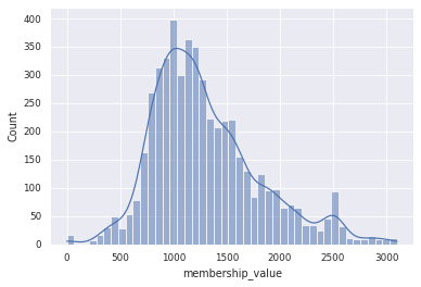
Depending on the distance cutoffs, we can assign our BGCs to a different numbers of GCF model. The default cutoffs is 900 (run 6). In our data, 382 out of 515 BGCs can be assigned to 114 BiG-FAM GCF. Do note that the number of assigned GCF can be smaller if we only consider the first hit (the query returns 10 hits).
Smaller number means a closer distance to the GCF model. For further analysis, we will stick with the default cutoff.
A closer look to BiG-FAM distributions
BGCflow already cleans the data for downstream processing. The processed bigslice query can be found in bgcflow/data/processed/s_venezuelae/bigslice/query_as_6.0.1/.
data = pd.read_csv(bigslice_query_processed / "query_network.csv")
plot_overview(data)
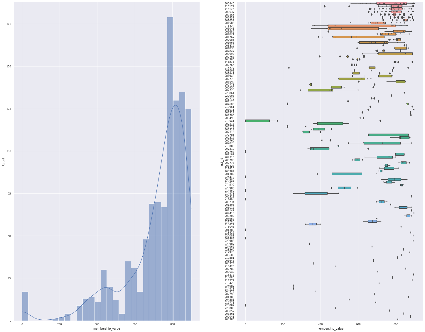
<Figure size 1800x1800 with 0 Axes>
On the figure above, we can see the distance distribution of our query to the model, and how each models have varying degree of distances. But, this data includes the top 10 hits, so 1 BGCs can be assigned to multiple GCFs.
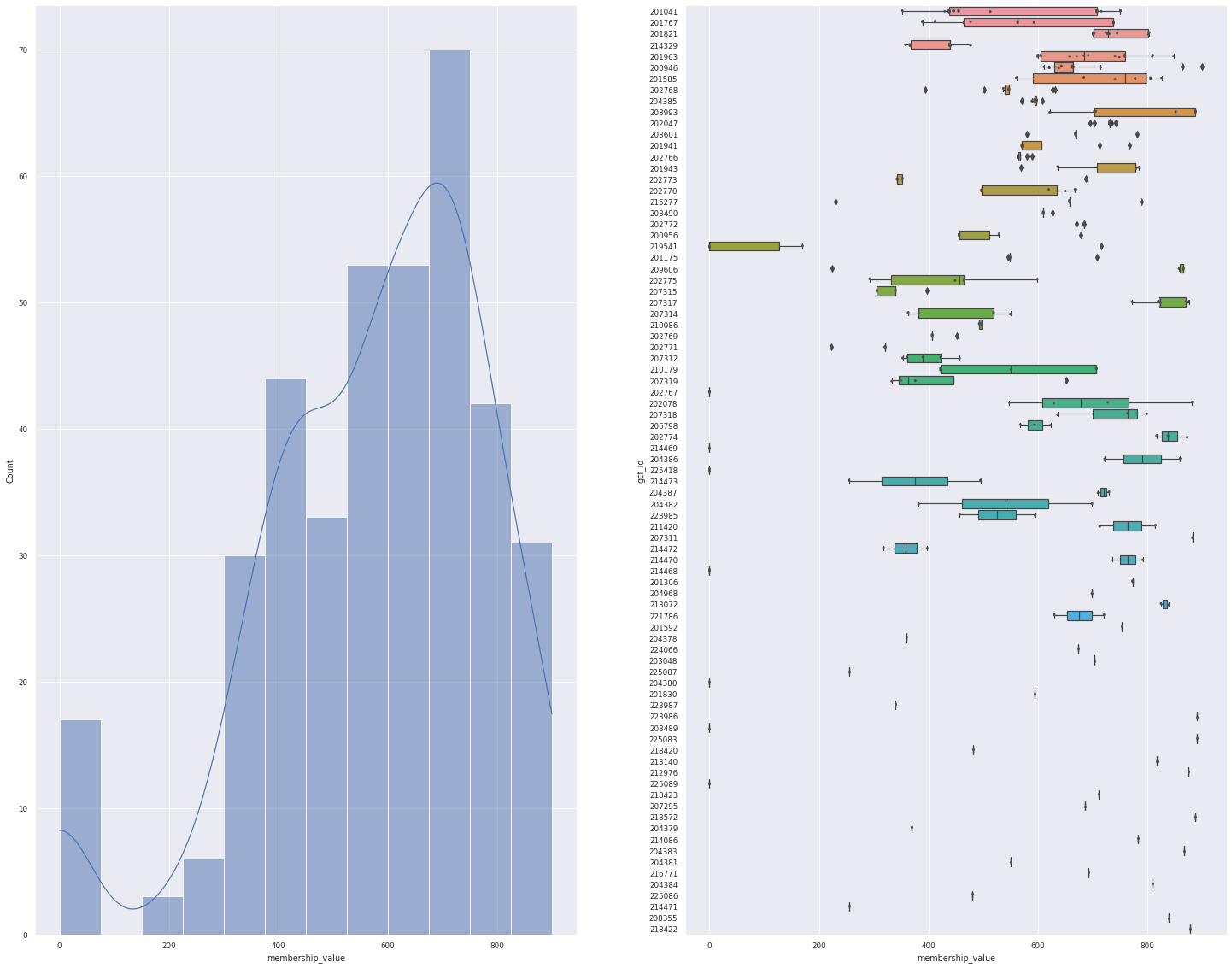
Let’s see again only for the first hit.
n_hits = 1 # get only the first hit
n_hits_only = data.loc[:, "rank"].isin(np.arange(n_hits))
data_1 = data[n_hits_only]
print(f"For the top {n_hits} hit, {len(data_1.bgc_id.unique())} BGCs can be mapped to {len(data_1.gcf_id.unique())} GCF")
plot_overview(data_1)
For the top 1 hit, 382 BGCs can be mapped to 83 GCF
<Figure size 1800x1800 with 0 Axes>
Annotate Network with information from BiG-SCAPE and GTDB
These network will only be meaningful when we enrich it with metadata. We can use information from our BiG-SCAPE runs, taxonomic information from GTDB-tk, and other tables generated by BGCflow.
# Enrich with BiG-SCAPE
df_annotation = pd.read_csv(bigscape_result, index_col=0)
df_annotation.loc[:, "bigslice_query"] = "query"
for i in data["gcf_id"].unique():
    df_annotation.loc[i, "bigslice_query"] = "model"

# enrich with GTDB
df_gtdb = pd.read_csv(gtdb_table).set_index("genome_id")
for i in df_annotation.index:
    genome_id = df_annotation.loc[i, "genome_id"]
    if type(genome_id) == str:
        for item in ["gtdb_release", "Domain", "Phylum", "Class", "Order", "Family", "Genus", "Species", "Organism"]:
            df_annotation.loc[i, item] = df_gtdb.loc[genome_id, item]

# enrich with bgc info - will be put in the main bgcflow code
bgc_info = df_bgc.copy()
bgc_info["bgc_id"] = [str(i).replace(".gbk", "") for i in bgc_info["orig_filename"]]
bgc_info = bgc_info.set_index("bgc_id")
for i in df_annotation.index:
    try:
        df_annotation.loc[i, "on_contig_edge"] = bgc_info.loc[i, "on_contig_edge"]
        df_annotation.loc[i, "length_nt"] = bgc_info.loc[i, "length_nt"]
    except KeyError:
        pass
df_annotation.head()
| product | bigscape_class | genome_id | accn_id | gcf_0.30 | gcf_0.40 | gcf_0.50 | Clan Number | fam_id_0.30 | fam_type_0.30 | ... | Domain | Phylum | Class | Order | Family | Genus | Species | Organism | on_contig_edge | length_nt | |
|---|---|---|---|---|---|---|---|---|---|---|---|---|---|---|---|---|---|---|---|---|---|
| NC_018750.1.region001 | ectoine | Others | GCF_000253235.1 | NC_018750.1 | 1911.0 | 1911.0 | 1911.0 | 2045.0 | 2.0 | known_family | ... | d__Bacteria | p__Actinobacteriota | c__Actinomycetia | o__Streptomycetales | f__Streptomycetaceae | g__Streptomyces | venezuelae | s__Streptomyces venezuelae | 0.0 | 10417.0 |
| NC_018750.1.region002 | terpene | Terpene | GCF_000253235.1 | NC_018750.1 | 2109.0 | 2109.0 | 2109.0 | NaN | 14.0 | unknown_family | ... | d__Bacteria | p__Actinobacteriota | c__Actinomycetia | o__Streptomycetales | f__Streptomycetaceae | g__Streptomyces | venezuelae | s__Streptomyces venezuelae | 0.0 | 20954.0 |
| NC_018750.1.region003 | T3PKS.NRPS.NRPS-like.T1PKS | PKS-NRP_Hybrids | GCF_000253235.1 | NC_018750.1 | 1913.0 | 1913.0 | 1913.0 | NaN | 22.0 | known_family | ... | d__Bacteria | p__Actinobacteriota | c__Actinomycetia | o__Streptomycetales | f__Streptomycetaceae | g__Streptomyces | venezuelae | s__Streptomyces venezuelae | 0.0 | 99490.0 |
| NC_018750.1.region004 | terpene.lanthipeptide-class-ii | Others | GCF_000253235.1 | NC_018750.1 | 2111.0 | 2111.0 | 2111.0 | 36.0 | 20.0 | unknown_family | ... | d__Bacteria | p__Actinobacteriota | c__Actinomycetia | o__Streptomycetales | f__Streptomycetaceae | g__Streptomyces | venezuelae | s__Streptomyces venezuelae | 0.0 | 29652.0 |
| NC_018750.1.region005 | lanthipeptide-class-iv | RiPPs | GCF_000253235.1 | NC_018750.1 | 2399.0 | 2399.0 | 2399.0 | 552.0 | 17.0 | known_family | ... | d__Bacteria | p__Actinobacteriota | c__Actinomycetia | o__Streptomycetales | f__Streptomycetaceae | g__Streptomyces | venezuelae | s__Streptomyces venezuelae | 0.0 | 22853.0 |
5 rows × 23 columns
df_annotation.to_csv("../tables/bigslice/enriched_query_annotation.csv")
Import the annotation to Cytoscape
Download the enriched_query_annotation.csv and import it to enrich the nodes in Cytoscape network.
Using the new annotations, play around and explore the network to find interesting BGCs and their BiG-FAM models.
Key Points
Different BGCflow outputs can be combined to enrich BiG-SLICE query network
Exploring BGCFlow result with MKDocs
Overview
Teaching: 5 min
Exercises: 0 minQuestions
How do I look at BGCFlow results?
Objectives
Starting an mkdocs server of BGCFlow results
Exploring and using BGCFlow Jupyter Notebooks template
Pre-requisite
- Activate the BGCFlow conda environment (see Part 1 - Introduction)
conda activate bgcflow
Getting a demo report
- Download an example report from Zenodo
wget -O Lactobacillus_delbrueckii_report.zip https://zenodo.org/record/7740349/files/Lactobacillus_delbrueckii_report.zip?download=1
unzip Lactobacillus_delbrueckii_report.zip
Starting BGCFlow mkdocs server
- Move to the report directory and use
bgcflow servecommand to start up a http file server and mkdocs:cd Lactobacillus_delbrueckii_report/Lactobacillus_delbrueckii bgcflow serve --project Lactobacillus_delbrueckii - The report can be accessed in http://localhost:8001/
Key Points
For each BGCFlow projects, the result is structured as an interactive Markdown documentation that can be modified
Reports are made using Jupyter notebooks running on Python or R environments
Exploring BGCFlow result database using Metabase
Overview
Teaching: 5 min
Exercises: 0 minQuestions
How do I explore and query tabular data from BGCFlow result?
Objectives
Start a local Metabase server
Loadi BGCFlow OLAP database (DuckDB) in metabase
Pre-requisite
- Activate the BGCFlow conda environment and make sure you have a clone of BGCFlow installed locally (see Part 1 - Introduction)
cd <your BGCFlow path> conda activate bgcflow - Download and extract a BGCFlow project demo (see Part 7)
Starting Metabase server
- Make sure you are in your bgcflow directory. Metabase can then be started using:
bgcflow serve --metabase - Metabase will be launched in locally in http://localhost:3000/
Setting a local Metabase account
- Follow the steps to set up your account
- Choose DuckDB as the database type and give the DuckDB Path:
/home/<my_user_name>/Lactobacillus_delbrueckii_report/Lactobacillus_delbrueckii/dbt_as_6.1.1/
Key Points
All of the tabular ouputs from BGCFlow are loaded and transformed into an OLAP database (DuckDB)
A business intelligence tools such as Metabase, can be used to interactively explore the database and build SQL queries
Customizing BGCFlow config for analyzing fungal genomes
Overview
Teaching: 5 min
Exercises: 0 minQuestions
How can I run BGCFlow for fungal genomes using a custom configuration?
Objectives
Understand how to customize BGCFlow configuration for fungal genomes
Learn how to run BGCFlow with a specific configuration for fungal genome analysis
Pre-requisite
- Activate the BGCFlow conda environment and make sure you have a clone of BGCFlow installed locally (see Part 1 - Introduction)
cd <your BGCFlow path>
git checkout dev-0.9.0-1
conda activate bgcflow
- Make sure to have the
bgcflow_wrapperversion0.3.5or above:
bgcflow --version
bgcflow_wrapper, version 0.3.5
Set up Fungi Project Configuration
- Inside the config folder, create a new project folder named fungi, the final project configuration will look like this:
config/
├── fungi
│   ├── project_config.yaml # BGCFlow project config
│   └── samples.csv # a csv files listing all your samples
└── config.yaml # BGCFlow global config
- Create the
project_config.yamland edit the contain to have this values:
name: Fungi
pep_version: 2.1.0
description: "Example of a fungi project."
input_folder: "."
input_type: "gbk" # BGCFlow does not have annotation tools for eukaryotes, so we will use the genbank from NCBI
sample_table: samples.csv

#### RULE CONFIGURATION ####
# rules: set value to TRUE if you want to run the analysis or FALSE if you don't
rules:
  seqfu: TRUE
  mash: TRUE
  fastani: FALSE
  checkm: FALSE
  gtdbtk: FALSE
  prokka-gbk: FALSE
  antismash: TRUE
  query-bigslice: TRUE
  bigscape: TRUE
  bigslice: TRUE
  automlst-wrapper: FALSE
  arts: FALSE
  roary: FALSE
  eggnog: TRUE
  eggnog-roary: FALSE
  deeptfactor: FALSE
  deeptfactor-roary: FALSE
  cblaster-genome: TRUE
  cblaster-bgc: TRUE
- Please note that some tools are not designed for for analysing fungal genomes.
- Create or edit
samples.csvto have this values:
genome_id,source,organism,genus,species,strain,closest_placement_reference,input_file
GCA_014117465.1,ncbi,,,,,,
GCA_014784225.2,ncbi,,,,,,
GCA_030515275.1,ncbi,,,,,,
GCA_014117485.1,ncbi,,,,,,
Update the global configuration
- Now that we have our project ready, we need to update the global configuration so it is registered as one of the BGCFlow project to run
- Edit the
config/config.yamlfile to include only the fungal project to run:
# This file should contain everything to configure the workflow on a global scale.

#### PROJECT INFORMATION ####
# This section control your project configuration.
# Each project are separated by "-".
# A project can be defined as (1) a yaml object or (2) a Portable Encapsulated Project (PEP) file.
# (1) To define project as a yaml object, it must contain the variable "name" and "samples".
#   - name : name of your project
#   - samples : a csv file containing a list of genome ids for analysis with multiple sources mentioned. Genome ids must be unique.
#   - rules: a yaml file containing project rule configurations. This will override global rule configuration.
#   - prokka-db (optional): list of the custom accessions to use as prokka reference database.
#   - gtdb-tax (optional): output summary file of GTDB-tk with "user_genome" and "classification" as the two minimum columns
# (2) To define project using PEP file, only variable "name" should be given that points to the location of the PEP yaml file.
#   - pep: path to PEP .yaml file. See project example_pep for details.
# PS: the variable pep and name is an alias

projects:
# Project 2 (PEP file)
  - pep: config/fungi/project_config.yaml

bgc_projects:
  - pep: config/lanthipeptide_lactobacillus/project_config.yaml
...
Running the main BGCFlow pipeline
- Run the workflow by changing the config by:
snakemake --use-conda -c 8 --config "taxonomic_mode=fungi"
Key Points
BGCFlow can be customized for analyzing fungal genomes using specific configurations
Running BGCFlow with these configurations allows for targeted analysis of fungal genomes